
Building Footprints Comparison: SAM 3 vs ESRI
Extracted building outlines across Lewisville, Texas, from 21.1 gigapixels of 10 cm Nearmap imagery with Meta’s SAM 3 and Esri’s pretrained Mask R-CNN, then compared them with identical cleanup and scoring, a tuning protocol written in advance, and a test area scored once.
Project gallery
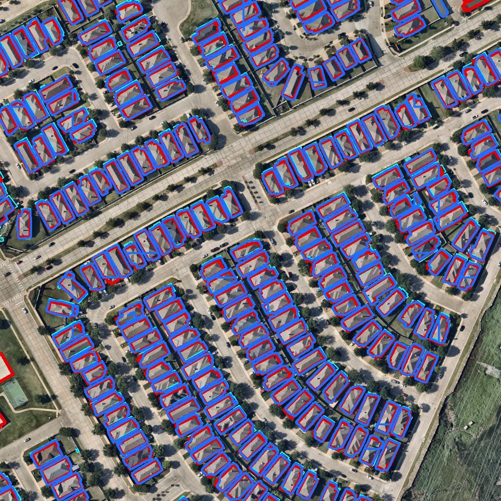
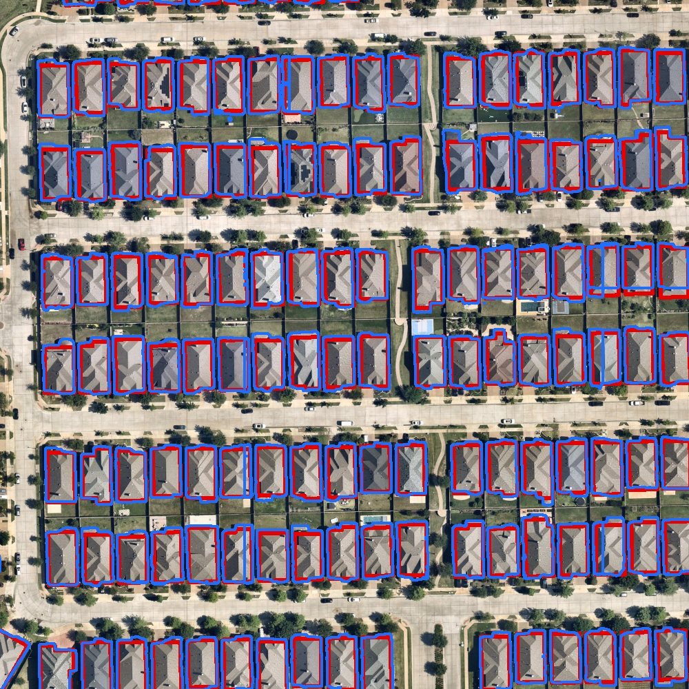
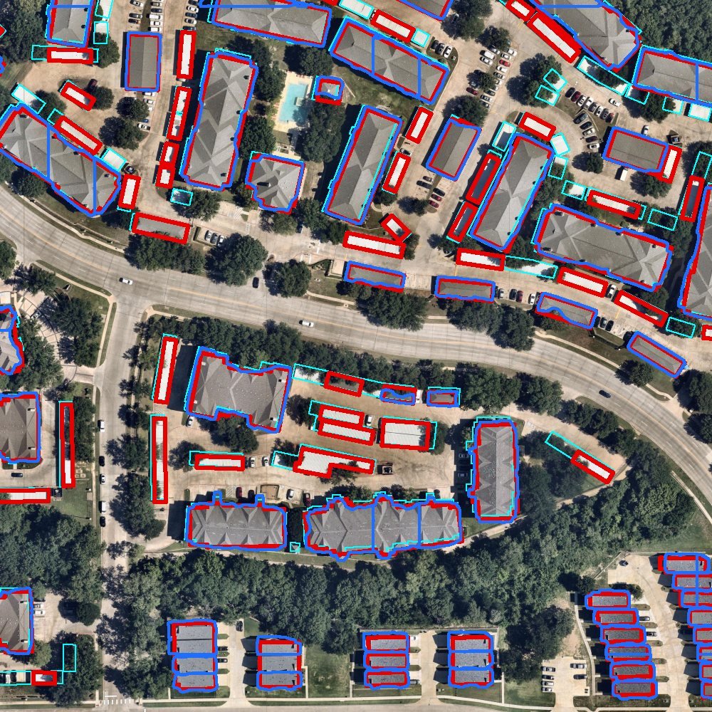
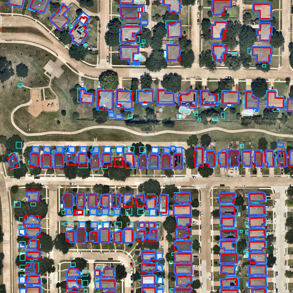
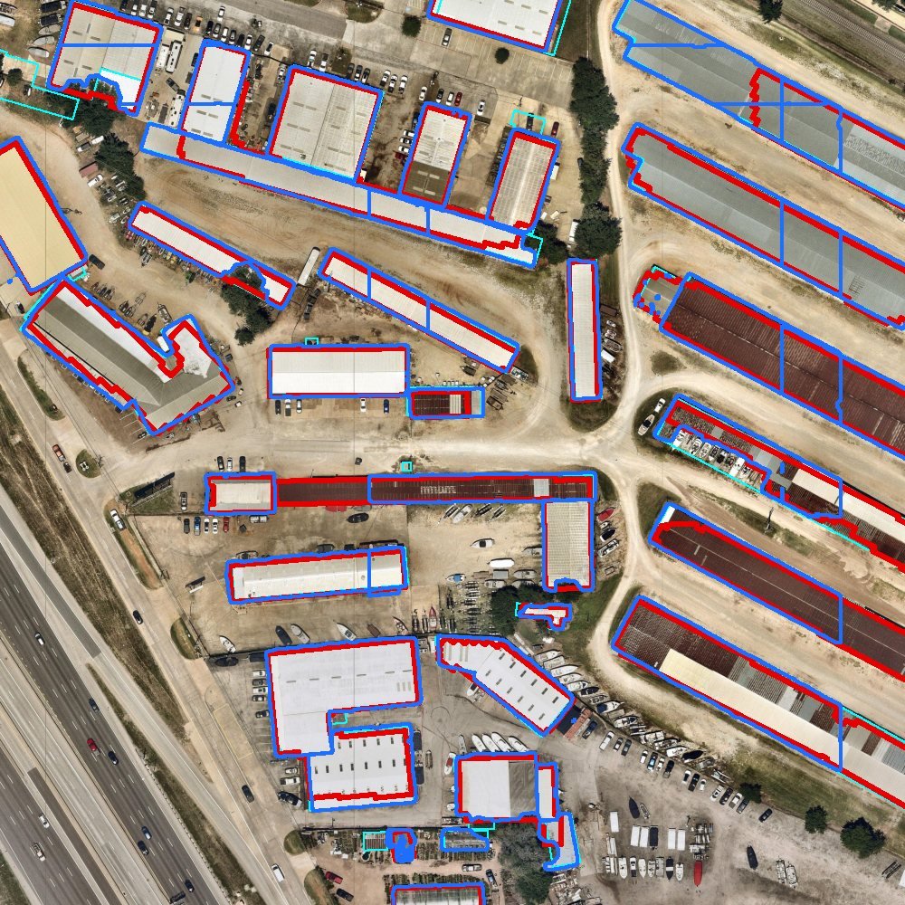
Aerial imagery: Nearmap, May 2026. Red is Esri, blue is SAM 3, thin cyan is the city’s 2015 outlines. 5 images. Select an image to view it full size.
My contribution
I built the nbf toolkit and the evaluation. I ran SAM 3 across the city and ran Esri’s model locally, then scored both alongside the Esri run the city published, using the same cleanup and scoring rules. I did not train or fine-tune either model, and the scores measure agreement with the city’s 2015 building outlines, not accuracy.
Result: On main buildings of 20 m² and up, Esri’s city run agrees best with the city’s 2015 outlines: city-wide F1 0.83 vs 0.74 for SAM 3. Scored once on the test area, F1 is 0.95 for Esri’s city run, 0.91 for Esri’s local run, and 0.87 for SAM 3. SAM 3 processed the whole city in 2 h 41 min on a 6 GB laptop GPU (RTX 4050).
Tools
- Python 3.12 and 3.13
- PyTorch 2.10 with CUDA 12.8
- SAM 3 through SamGeo 1.4.2
- ArcGIS Pro 3.7 and ArcPy (Image Analyst)
- rasterio and GDAL
- GeoPandas, Shapely 2, pyproj
- SciPy
- WSL2
- pytest, coverage, ruff
- GitHub Actions
- Jupyter
Agreement, not accuracy: every score is measured against the city’s 2015 building outlines, which are years older than the imagery. Neither model finds most sheds under 20 m², and both split very large buildings at processing boundaries.
Approach
A comparison of two ways to extract building outlines from aerial imagery, run across an entire city: Meta’s SAM 3, a foundation model prompted with the word “building”, and Esri’s pretrained Building Footprint Extraction – USA model, a Mask R-CNN. Both ran over 21.1 gigapixels of 10 cm Nearmap imagery of Lewisville, Texas, and went through the same cleanup, scoring and tuning rules.
- Imagery preparation: the 25 GB mosaic declared a local coordinate system in metres; its numbers were really Texas State Plane in US survey feet. A small VRT relabels it without resampling a pixel. The city was then cut into 6,538 overlapping tiles with a hash-checked manifest.
- SAM 3: ran on a 6 GB laptop GPU under WSL2, tile by tile, with per-tile receipts so an interrupted run resumes where it stopped. Scores were kept from 0.3 upward, so any cut-off could be applied later without rerunning the model.
- Esri: ran through ArcGIS Pro in 150 overlapping chunks. Each chunk owns a core, so the merge never double-counts, and ArcGIS restarts every 8 chunks because its GPU memory grew until the model failed to load.
- The same scoring for every method: geometry repair, duplicate suppression that keeps the complete copy of a building cut at a tile seam, and one-to-one matching at IoU ≥ 0.5.
- Honest labels: every report declares whether its reference is an independent holdout or an older inventory. Here it is the older inventory, so every score is agreement, not accuracy.
- Tuning without peeking: the objective and the selection rule were written down before tuning. 176 variants were scored on one area, a documented amendment extended the cut-off range, and the frozen settings were scored once on a randomly chosen test area. The code refuses to score that area twice.

Results
| Measure | Esri, city run | Esri, local raw run | SAM 3 |
|---|---|---|---|
| City-wide F1 | 0.83 | 0.77 | 0.74 |
| City-wide precision / recall | 0.82 / 0.85 | 0.70 / 0.84 | 0.68 / 0.82 |
| Test-area F1, scored once | 0.95 | 0.91 | 0.87 |
| Structures under 20 m² found, of 7,867 | 2 | 352 | 267 |
| Run time, whole city | published by the city | 8 h 46 min | 2 h 41 min |
What the scores say
- Esri’s published run agrees best with the 2015 outlines, mostly on precision. Its own post-processing matters: the same model run locally without it scores 0.77.
- The two models mostly agree: 91% of Esri’s outlines have a matching SAM 3 outline, and matched outlines from SAM 3 fit slightly more tightly (median IoU 0.80 against 0.77).
- Many “extra” outlines are real: 4,923 SAM 3 outlines with no 2015 counterpart are also drawn by Esri, including whole subdivisions built since 2015.
- Neither model finds sheds, and both split very large buildings at processing boundaries.

Found by both, one model, or neither

Engineering highlights
- A Python toolkit and CLI, nbf, covering inspection, tiling, SAM 3 inference, Esri runs and imports, cleanup, evaluation, comparison and training-data preparation.
- Resumable, hash-verified inference: a changed tile or output is refused, not silently reused.
- GPU memory growth inside ArcGIS, found mid-run, handled by restarting its Python every 8 chunks, with no chunk lost or counted twice.
- Evaluation with maximum-cardinality one-to-one matching, row-order fingerprints that tie every result to its exact inputs, and per-building comparison across methods.
- 151 automated tests in CI on Windows and Ubuntu with Python 3.12 and 3.13, and four walkthrough notebooks executed end to end: SAM 3 on the GPU, Esri through ArcGIS Pro.
Limitations and next steps
- Agreement, not accuracy: the reference outlines are years older than the imagery. Review packages for two sample areas are ready; scoring the frozen settings against reviewed outlines needs no further tuning.
- Small structures: no model finds most sheds under 20 m²; that would take fine-tuning on labelled examples.
- Large buildings: merging outlines across tile seams would stop long roofs from being split.
Earlier groundwork: collecting the imagery at scale
Before this comparison, I built an imagery collection and mosaic workflow for an October 2025 Nearmap collection, then ran deep-learning extraction of building footprints and roads on the prepared imagery. That collection predates the May 2026 imagery used in the comparison above; it is earlier work on the same problem, not an input to these scores.
I separated downloading, coverage checks, and mosaic assembly so a failed tile did not require repeating the entire collection. Recovery passes used the missing-tile list while keeping the files already collected. The counts below measure imagery coverage, not building or road extraction accuracy.
- October 9, 2025, initial download: 119,973 tiles saved; 453 missing, blank, or failed.
- October 13, 2025, recovery pass: 389 additional tiles saved; 64 still unresolved.
- October 14, 2025, final recovery pass: the last outstanding tile saved; zero unresolved after successive passes.
- October 14, 2025, coverage check: all 120,426 expected tiles present, with zero missing or undersized files, followed by a logged mosaic write.
- GDAL assigned tile bounds, combined the tiles through virtual rasters, clipped the mosaic to the boundary, and wrote tiled GeoTIFF output with overviews.

Technical details
Professional · Geospatial Software Developer / Data Scientist · Nearmap imagery, May 2026
Cities keep building inventories for permits, taxes and planning, and they go stale: Lewisville’s outlines date from 2015 or earlier. New aerial imagery arrives every year. The question was how a general-purpose foundation model compares with a purpose-built vendor model on the same imagery, and how to make that comparison fair and honest when the only reference outlines are years older than the imagery.
- Fix the imagery’s coordinate system through a VRT, then cut it into 6,538 tiles of 1,536 px with a hash-checked manifest.
- Run SAM 3, prompted with the word “building”, and Esri’s Mask R-CNN over the same imagery.
- Put both outputs through the same cleanup and scoring.
- Tune and freeze settings on one area, then score a randomly chosen test area once.